[ML] Dimensionality Reduction

Before implementing these dimensionality reduction algorithm, try to do whatever you want with the raw data first. In other words, please give yourself a good reason to add more complexity.

PCA - Principal Component Analysis

Problem formulation:
Reduce from n-dimension to k-dimension: Find \( k \) vectors \( u^{(1)}, u^{(2)}, …, u^{(k)} \) onto which to project the data, so as to minimize the projection error and reduce the risk of overfitting as well.

Usually the data should be preprocessed by Feature Scaling / Mean Normalization.

1. Compute “covariance matrix”:

\[ {\tiny \sum} = \frac{1}{m} \sum_{i = 1}^{n} (x^{(i)}) (x^{(i)})^{T} \]

1. Compute “eigenvectors” of matrix \(\tiny \sum \)

2. Project the raw data onto the k-dimensional space.

But how to choose \( k \)?

Typically, choose \( k \) to be the smallest value so that:

\[ \frac{\frac{1}{m} \sum_{i=1}^{m} \parallel x^{(i)} - x_{approx}^{(i)} \parallel ^2 } {\frac{1}{m} \sum_{i=1}^{m} \parallel x^{(i)} \parallel^2 } \leq 0.01 (0.05) \]

In other words, “99%/95% of the variance is retained.”

Note:
Run PCA just on your training data and apply the mapping to the cross validation data set and test data set.

SVD:
SVD(Singular Value Decomposition) is another form of PCA, there’s no significant distinctions between these two.

LDA - Linear Discriminant Analysis

Both LDA and PCA are linear transformation techniques: LDA is supervised whereas PCA is unsupervised (ignores class labels).

If PCA finds the dimensions that explain the most overall variance, then LDA finds the dimensions that explain the most variance which can separate different classes the best.

Further note that the number of eigenvalues in LDA is \( min(num_groups-1,num_features) \).

The reason comes from the in-between class scatter matrix. We create it by adding \( c \) (\( c \) =number of classes) matrices that have rank 1 or less, so we can only have c-1 non-zero eigenvalues at max. But we’ll skip the implementation details here.

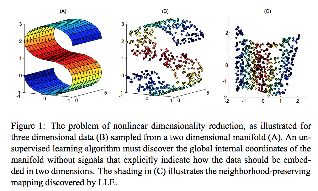
LLE - Locally Linear Embedding

LLE is an important non-linear dimensionality reduction method. It can preserve the original “shape” of the data to lower dimensions.

1. It begins by finding a set of the nearest neighbors of each point.

2. It then computes a set of weights for each point that best describes the point as a linear combination of its neighbors.

3. Finally, it uses an eigenvector-based optimization technique to find the low-dimensional embedding of points, such that each point istill described with the same linear combination of its neighbors.

But LLE tends to handle non-uniform sample densities poorly because there is no fixed unit to prevent the weights from drifting as various regions differ in sample densities. LLE has no internal model.

LE - Laplacian Eigenmap

Laplacian Eigenmaps uses spectral techniques to perform dimensionality reduction. This technique relies on the basic assumption that the data lies in a low-dimensional manifold in a high-dimensional space. This algorithm cannot embed out of sample points.

Traditional techniques like principal component analysis do not consider the intrinsic geometry of the data. Laplacian eigenmaps builds a graph from neighborhood information of the data set. Each data point serves as a node on the graph and connectivity between nodes is governed by the proximity of neighboring points (using e.g. the k-nearest neighbor algorithm). The graph thus generated can be considered as a discrete approximation of the low-dimensional manifold in the high-dimensional space.