[ML] Naive Bayes
Difference between “Naive Bayes” and “Bayesian Networks”
According to Omkar Lad:
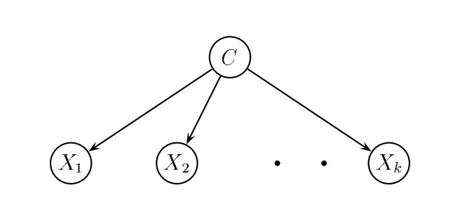
Naive Bayes assumes that all the features are conditionally independent of each other. This therefore permits us to use the Bayesian rule for probability. Usually this independence assumption works well for most cases, if even in actuality they are not really independent.
Bayesian network does not have such assumptions. All the dependence in Bayesian Network has to be modeled. The Bayesian network (graph) formed can be learned by the machine itself, or can be designed in prior, by the developer, if he has sufficient knowledge of the dependencies.
That is to say, a “Naive” Bayes is actually a special case of Bayesian Networks.
Details
As introduced in the blog titled Bayesian Methods Overview, we have the following equations as the heart of the method:
\[P(\theta|X) = \frac{P(X,\theta)}{P(X)} = \frac{P(X|\theta)P(\theta)}{P(X)}\]But given the training data, how to compute \( P(X \vert \theta) \) is not clearly specified. Actually, we have two major ways to do this depending on the type of the data we have:
Discrete feature: we can simply compute the likelihood using the table.
Continuous feature:
- Discretize numeric variables: this is to split the data into several categories and treat them as discrete features.
- Use Probability Density Functions(PDFs): this is to assume the probability distribution for an attribute follows a normal or Gaussian distribution(Gaussian Naive Bayes). But if it is known to follow some other distribution, such as Poisson’s, then the equivalent probability density function can be used.
For continuous feature, we compute its mean and standard deviation to come up with the PDF we assume.